Forecast accuracy is a criterion for evaluating how suitable a particular forecasting method might be for a particular data set. Forecast accuracy is the main reason to select one forecast model over another. Forecast accuracy is also the reason to tune the parameters for a given model. Forecast accuracy refers to how well a current forecasting model is able to reproduce the data that is already known.
Six measures of forecasting accuracy are defined and quantified: MAE, ME, MAPE, PVE, Tracking signal, and Theil's U-statistic. In addition to these R Bar Squared is also available when running one of the regression models. Forecast models can be evaluated based on the value of one or more of these measures.
|
n |
Number of observations. |
|
Dt |
Observed demand in period t. |
|
Ft |
Forecast in period t. |
|
D |
Delta (tracking signal smoothing parameter). |
|
et |
= Dt.- Ft |
The available measures are:
MAE is an abbreviation for mean absolute error. The formula is as follows:
![]()
This formula is run from the latest historical period, and the number of periods specified in the forecast error periods back in time (n=forecast error periods). (See Demand Plan Server Setup/General)
The value of MAE is MAE multiplied by the inventory value for the item. Forecasted items with the highest value of MAE are the most profitable candidates for better accuracy.
ME is an abbreviation for mean error. The formula is as follows:
![]()
ME criteria are likely to be limited since positive and negative errors tend to offset one another. In fact, the ME will only tell if there is systematic under- or over-forecasting, also called the forecast bias. This formula is run from the latest historical period, and the number of periods specified in the forecast error periods back in time (n=forecast error periods). (See Demand Plan Server Setup/General)
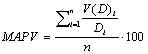
MAPE is an abbreviation for mean absolute percentage error, The formula is as follows:
MAPE expresses the relative inaccuracy in the forecast for each item. Items with the highest MAPE should benefit from increased forecast accuracy. This formula is run from the latest historical period, and the number of periods specified in the forecast error periods back in time (n=forecast error periods). (See Demand Plan Server Setup/General)
WMAPE is an abbreviation for weighted mean absolute percentage error, The formula is as follows:

WMAPE expresses the relative inaccuracy in the forecast for each item. Where periods with large abs errors are given more weight than periods with small abs errors. This does not allow periods that have small abs errors but huge percentage errors do dominate the measurement. Items with the highest WMAPE should benefit from increased forecast accuracy. This formula is run from the latest historical period, and the number of periods specified in the forecast error periods back in time (n=forecast error periods). (See Demand Plan Server Setup/General)
MSE is an abbreviation for mean squared error, The formula is as follows:
![]()
MSE expresses the squared inaccuracy in the forecast for each item. Items with the highest MSE should benefit from increased forecast accuracy. MSE has the property that parts with single large forecast errors gets more penalized than a part that has a equal forecast error but with the errors more evenly distributed over the measurement period. This formula is run from the latest historical period, and the number of periods specified in the forecast error periods back in time (n=forecast error periods). (See Demand Plan Server Setup/General)
PVE is an abbreviation for percentage variation explained. The formulas are as follows:

![]()
![]()
PVE indicates what portion of the inherent variation in the demand being explained by the forecast model. PVE shows if the forecast is getting better or worse over time since it adjusts for changes in demand volatility. It is also a good benchmarking measure. If PVE is less than zero the forecast is actually increasing the variation of the demand. In this case, change the forecast model used or adjust the parameters (increase alpha, or number of moving average periods).
This formula is run from the latest historical period, and the number of periods specified in the forecast error periods back in time (n=forecast error periods). (See Demand Plan Server Setup/General)
The tracking signal is a means of monitoring the bias and reacting to changes in the demand pattern. A high tracking signal (i.e., > 0.6) suggests that there is a systematic error or bias in the forecast. The lower the delta value the less risk for false alarms (the alarm goes off later than with a high delta). A delta value between 0.1 and 0.3 is recommended. The formulas are as follows:
![]()
![]()
![]()
This formula is run from the latest historical period, and the number of periods specified in the forecast error periods back in time (n=forecast error periods). (See Demand Plan Server Setup/General)
Adjustment Factor, The formula is as follows:
![]()
![]()
![]()
Adjustment factor expresses difference between the users adjusted forecast (historical forecast) and a pure mathematical forecast (explanation forecast), an adjustment factor of 10 means the user adjusted forecast i 10% more accurate than the pure mathematical forecast, -10 means that the pure mathematical one are better. Items with the high negative adjustment factor should benefit from a pure mathematical forecast (hands off). This formula is run from the latest historical period, and the number of periods specified in the forecast error periods back in time (n=forecast error periods). (See Demand Plan Server Setup/General)
This statistic enables you to make a relative comparison of the selected formal forecasting methods simple approaches. The most naive approach is to specify as a forecast for the next period the actual demand of the previous period (Level forecast with a = 1.0) or the naive forecast model. Using the naive approach, the simple forecast relative error equals the actual relative change in demand. The challenge for any formal forecasting method is to predict more accurately than the naive approach. The interpretation of the value of the U-statistic is:
U = 1: The naive method is as good as the forecasting model being evaluated.
U < 1: The forecasting model being used is better than the simple method.
U > 1: There is no point in using the formal forecasting method since the naive approach is better.
The formula is as follows:
Note the difference between Theil's and the other error measures is that the Theil's U-statistic uses the explanation forecast, whereas the other six use the historical forecast. Therefore, the Theil's value will change when you change forecast models or parameters.
This formula is run from the latest historical period, and the number of periods specified in the measurement periods back in time (n=measurement periods). (See Demand Plan Server Setup/General)
Also called R2. This measure is only used when the forecast model regression (least squares) or multiple regression is used. R Squared has a useful interpretation as the proportion of variance in the historical demand, explained (accounted for) by the regression (when least square model is used) or the selected explanation variables (when multiple regression is used).
Notation:
|
Yi |
Regression estimation of the Demand variable. |
|
Di |
The Demand variable. |
![]()
This measure is only used when the forecast model regression (least squares) or multiple regression is used. R Bar Squared is sometimes called Adjusted R2 or Adjusted R Squared. This is almost the same as R Squared only that it corrects for the degrees of freedom. R Bar Squared is commonly used to find the best regression model. The higher the R Bar Squared the better. R Bar Squared will however not always increase with the number of explanation variable (as R Square does), R Bar Squared only increases when the added explanation variable give added value to the regression.
Notation:
|
k |
The number of explanation variables |
|
Yi |
Regression estimation of the Demand variable. |
|
Di |
The Demand variable.> |