Designing an Advanced Report—Exercises
| IMPORTANT |
| The exercise scenarios in this document uses data from the RACE version
of the database released with App75 SP4 as example data. |
Creating a Chart using Microsoft Excel 2007
Purpose: The purpose of this exercise is to create a chart
for the report that was created in Design exercise.
Windows:
IFS Business Analytics/Go to Design
- Open the report DESIGNXX and click Go To Design
- Select cell C15 and select Insert menu from Microsoft Excel tool bar
and click Column and select 2D -Column.
- Right click in the chart area and click Select Data. Select cell
C13(=Sheet1$C$13) to chart data range.
- Click Ok.
- Right click and select Select Data. In the Horizontal Axis Labels click Edit.
- Enter C4(=Sheet1$C$4) in Axis Label Range
- Click Layout tab and Chart Title from Microsoft Excel tool bar and
enter "Net Profit per Period" as the title above the chart.
- Select layout and click Legend from Microsoft Excel toolbar. Select
None.
- Select Layout and click Data Labels from Microsoft Excel toolbar.
Select Center. Refer to the figure below:
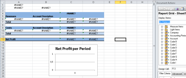
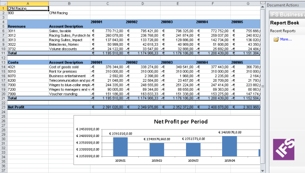
- Click Execute. The executed report should look like the figure
below:
Creating a Pivot Report
Purpose: The purpose of this exercise is to show you how
to create a report using the pivot feature in IFS Business Analytics.
Windows:
IFS Business Analytics/Go to Design/Pivot
- Create a new report using GL Balance and GL Period Budget information
sources.
- Select cell A1 and click Pivot. The pivot will be positioned
here.
- Select GL Balance information source and drag Balance from
Measure Items and Account, Account Description and Account
Type from Account dimension and Accounting Period from
Accounting Period dimension into
Select Display Items pane. (Display items can also be entered by
double clicking on each item)
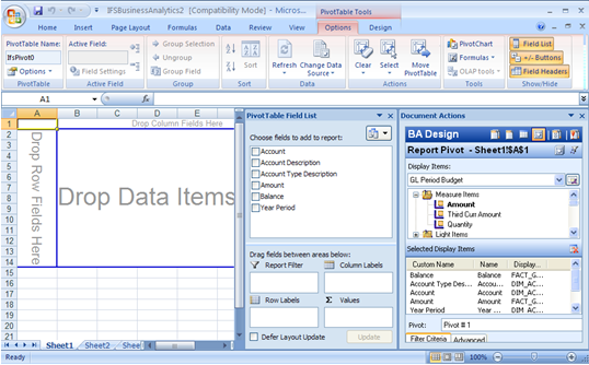
- Select GL Period Budget information source and and drag Amount
to the Display Items pane. Refer to the figure below:
- Select the Filter Criteria tab and drag the Display Items
where Company ="900", Account Type in "COST"; "REVENUE"
and Accounting Period
Between "200801" AND "200805".
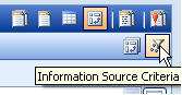
- Click Information Source Criteria as show in the figure below:
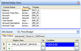
- Select GL Period Budget information source from the list and filter for
Budget Version "2010-B". Refer to the figure below:
- Drag the following Display Item and refer to the figure below:
Column Items: Year Period
Row Items: Account Type, Account, Account Description
Data Items: Balance Amount, Amount
Note: You can use normal Microsoft Excel Pivot functions to change headings
of columns and insert a formula and change the layout. This works differently
in Microsoft Excel 2003.
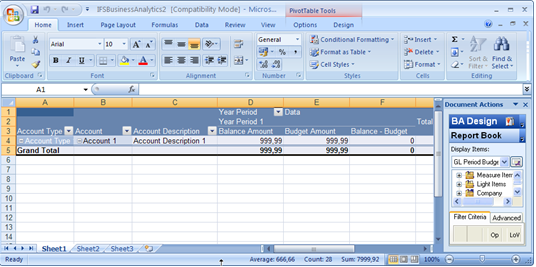
- The design should look something similar to the figure below:
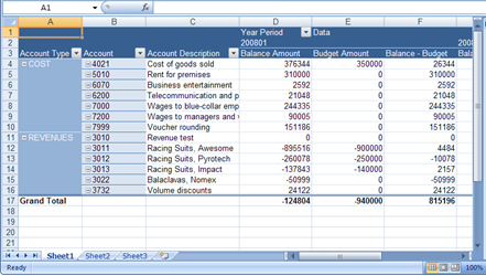
- Click Execute. The result should look similar to the figure
below:
- Save the report locally and name the file 'PIVOTXX' ( XX is your
initials)